Photogrammetry

In this section of the tutorial, you will construct a 3D model of a real world object using a technique known as photogrammetry.

Photogrammetry estimates the 3D geometric properties (such as shape, size, and positions of objects) of an object from 2D images taken from different perspectives. While this might sound like magic, it is based on well-established physical principles. These principles, at a high level, span:

• How camera captures light and projects it onto image sensor
• Algorithms that inferring camera spatial location at the time when images were captured
• Depth estimation from 2D images sequences
• 3D model reconstruction from color and depth information

This tutorial will provide practical experience using photogrammetry.

Setting up your workflow

Download Meshroom, along with this dataset to a Linux / Windows computer that has an Nvidia GPU.

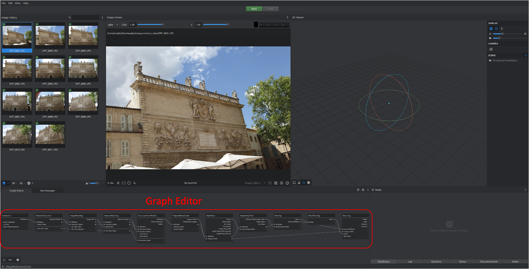
After opening Meshroom and loading the dataset, you should see an interface as shown below. The key thing to notice is the Graph Editor panel located in the bottom left. This panel describes individual steps that photogrammetry involves. To get to know the purpose of each step, read the AliceVision photogrammetry writeup.

Now, click start to generate your first 3D model. This will take several minutes or more depending on the compute power of your machine. After it’s finished, you should see sparse 3D point cloud shown in the 3D viewer panel:

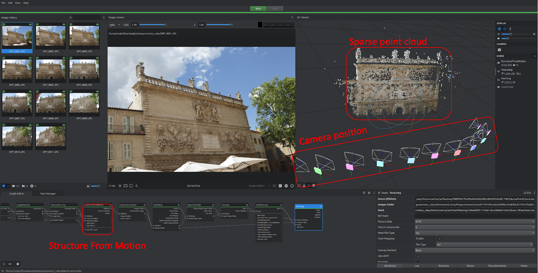
If you look closely at the Scene section in 3D Viewer, you’ll find this is actually showing sparse point cloud and estimated camera position generated from Structure From Motion step (one of the blocks in Graph Editor), we can toggle the eye icon to show/hide this view.

In fact, we can view output from many different steps in the viewer. Double clicking any blocks from Structure From Motion to Texturing will visualize the result. The final 3D model is generated at the Texturing step.

To access the final output files, right click on the Texturing node and select Open Folder. You’ll find one OBJ file that contains the 3D model, two EXR files that represent texture maps, and one MTL file that describes how the model and texture files link to each other.

Capture your own model

Now that you have reconstructed a model from the dataset, it’s time to collect your own data to build a model. All you need is to take images from multiple views (make sure there’s enough overlapping view between images) and re-execute the same workflow. Try to scan a real world object that has some animate-able features, as you will be adding animations to this scan later on.

This time, instead of running the pipeline only with default parameters in the nodes, explore how adjusting different parameters impacts the model quality. The knobs that might be of interest are:

• Texturing: Texture Size, Texture Downscale
• Mesh Decimate (right click to add this node): Simplification Factor

---

---